R in action读书笔记（12）第九章方差分析

jpld

13842

收藏 2015-04-27

第九章方差分析

9.2 ANOVA 模型拟合

9.2.1 aov()函数

aov(formula, data = NULL, projections =FALSE, qr = TRUE,

contrasts = NULL, ...)

9.2.2 表达式中各项的顺序

y ~ A + B + A:B

有三种类型的方法可以分解等式右边各效应对y所解释的方差。R默认类型I

类型I（序贯型）

效应根据表达式中先出现的效应做调整。A不做调整，B根据A调整，A:B交互项根据A和

B调整。

类型II（分层型）

效应根据同水平或低水平的效应做调整。A根据B调整，B依据A调整，A:B交互项同时根

据A和B调整。

类型III（边界型）

每个效应根据模型其他各效应做相应调整。A根据B和A:B做调整，A:B交互项根据A和B

调整。

9.3 单因素方差分析

> library(multcomp)

> attach(cholesterol)

> table(trt) #各组样本大小

trt

1time 2times4times drugD drugE

10 10 10 10 10

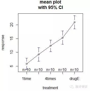
> aggregate(response,by=list(trt),FUN=mean)#各组均值

Group.1 x

1 1time 5.78197

2 2times 9.22497

3 4times 12.37478

4 drugD 15.36117

5 drugE 20.94752

> aggregate(response,by=list(trt),FUN=sd) #各组标准差

Group.1 x

1 1time 2.878113

2 2times 3.483054

3 4times 2.923119

4 drugD 3.454636

5 drugE 3.345003

> fit<-aov(response~trt)

> summary(fit) #检验组间差异（ANOVA）

Df SumSq Mean Sq F value Pr(>F)

trt 41351.4 337.8 32.43 9.82e-13 ***

Residuals 45 468.8 10.4

---

Signif. codes:

0 ‘***’ 0.001 ‘**’ 0.01 ‘*’ 0.05 ‘.’ 0.1 ‘ ’ 1

> library(gplots)

> plotmeans(response~trt,xlab="treatment",ylab="response",main="meanplot\nwith 95% CI")

#绘制各组均值及其置信区间的图形

> detach(cholesterol)

9.3.1 多重比较

TukeyHSD()函数提供了对各组均值差异的成对检验。但要注意TukeyHSD()函数与HH包存在兼容性问题：若载入HH包，TukeyHSD()函数将会失效。使用detach("package::HH")将它从搜寻路径中删除，然后再调用TukeyHSD()

> detach("package:HH", unload=TRUE)

> TukeyHSD(fit)

Tukey multiplecomparisons of means

95% family-wise confidence level

Fit: aov(formula = response ~ trt)

$trt

diff lwr upr p adj

2times-1time 3.44300 -0.6582817 7.5442820.1380949

4times-1time 6.59281 2.4915283 10.6940920.0003542

drugD-1time 9.57920 5.4779183 13.680482 0.0000003

drugE-1time 15.16555 11.0642683 19.266832 0.0000000

4times-2times 3.14981 -0.9514717 7.2510920.2050382

drugD-2times 6.13620 2.0349183 10.2374820.0009611

drugE-2times 11.72255 7.6212683 15.8238320.0000000

drugD-4times 2.98639 -1.1148917 7.0876720.2512446

drugE-4times 8.57274 4.4714583 12.6740220.0000037

drugE-drugD 5.58635 1.4850683 9.687632 0.0030633

> par(las=2)

> par(mar=c(5,8,4,2))

> plot(TukeyHSD(fit))

multcomp包中的glht()函数提供了多重均值比较更为全面的方法，既适用于线性模型，也适用于广义线性模型.

> library(multcomp)

> par(mar=c(5,4,6,2))

> tuk<-glht(fit,linfct=mcp(trt="Tukey"))

> plot(cld(tuk,level=.5),col="lightgrey")

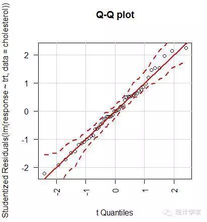
9.3.2 评估检验的假设条件

> library(car)

> qqPlot(lm(response~trt,data=cholesterol),simulate=TRUE,main="Q-Qplot",labels=FALSE)

Bartlett检验:

> bartlett.test(response~trt,data=cholesterol)

Bartlett test ofhomogeneity of variances

data: response by trt

Bartlett's K-squared = 0.5797, df = 4,

p-value = 0.9653

方差齐性分析对离群点非常敏感。可利用car包中的outlierTest()函数来检测离群点：

> library(car)

> outlierTest(fit)

No Studentized residuals withBonferonni p < 0.05

Largest |rstudent|:

rstudent unadjusted p-value Bonferonni p

19 2.251149 0.029422 NA

9.4 单因素协方差分析

单因素协方差分析（ANCOVA）扩展了单因素方差分析（ANOVA），包含一个或多个定量的

协变量

> data(litter,package="multcomp")

> attach(litter)

> table(dose)

dose

0 5 50 500

20 19 18 17

> aggregate(weight,by=list(dose),FUN=mean)

Group.1 x

1 0 32.30850

2 5 29.30842

3 50 29.86611

4 500 29.64647

> fit<-aov(weight~gesttime+dose)

> summary(fit)

Df Sum Sq Mean Sq Fvalue Pr(>F)

gesttime 1 134.3 134.30 8.049 0.00597 **

dose 3 137.1 45.71 2.739 0.04988 *

Residuals 69 1151.3 16.69

---

Signif. codes:

0 ‘***’ 0.001 ‘**’ 0.01 ‘*’ 0.05 ‘.’0.1 ‘ ’ 1

由于使用了协变量，要获取调整的组均值——即去除协变量效应后的组均值。可使

用effects包中的effects()函数来计算调整的均值：

> library(effects)

> effect("dose",fit)

dose effect

dose

0 5 50 500

32.35367 28.87672 30.56614 29.33460

对用户定义的对照的多重比较

> library(multcomp)

> contrast<-rbind("no drugvs. drug"=c(3,-1,-1,-1))

> summary(glht(fit,linfct=mcp(dose=contrast)))

Simultaneous Tests for General LinearHypotheses

Multiple Comparisons of Means: User-definedContrasts

Fit: aov(formula = weight ~ gesttime +dose)

Linear Hypotheses:

Estimate Std. Error tvalue

no drug vs. drug == 0 8.284 3.209 2.581

Pr(>|t|)

no drug vs. drug == 0 0.012 *

---

Signif. codes:

0 ‘***’ 0.001 ‘**’ 0.01 ‘*’ 0.05 ‘.’0.1 ‘ ’ 1

(Adjusted p values reported --single-step method)

9.4.1 评估检验的假设条件

检验回归斜率的同质性

> library(multcomp)

> fit2<-aov(weight~gesttime*dose,data=litter)

> summary(fit2)

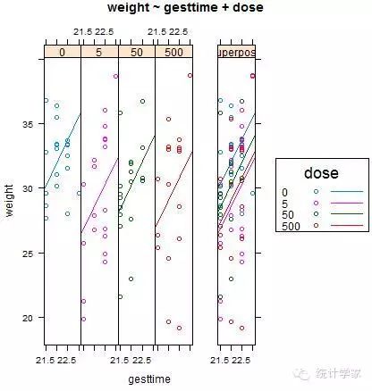
9.4.2 结果可视化

HH包中的ancova()函数可以绘制因变量、协变量和因子之间的关系图。

> library(HH)

> ancova(weight~gesttime+dose,data=litter)

扫码加我拉你入群

请注明：姓名-公司-职位

以便审核进群资格，未注明则拒绝

全部回复

jpld

2015-4-27 09:42:32

9.5 双因素方差分析
双因素ANOVA
> attach(ToothGrowth)
> table(supp,dose)
dose
supp 0.5  1  2
OJ  10 10 10
VC  10 10 10
> aggregate(len,by=list(supp,dose),FUN=mean)
Group.1 Group.2    x
1    OJ    0.5 13.23
2    VC    0.5  7.98
3    OJ    1.0 22.70
4    VC    1.0 16.77
5    OJ    2.0 26.06
6    VC    2.0 26.14
> aggregate(len,by=list(supp,dose),FUN=sd)
Group.1 Group.2       x
1    OJ    0.5 4.459709
2    VC    0.5 2.746634
3    OJ    1.0 3.910953
4    VC    1.0 2.515309
5    OJ    2.0 2.655058
6    VC    2.0 4.797731
> fit<-aov(len~supp*dose)
> summary(fit)
         Df Sum Sq Mean Sq F value Pr(>F)
supp       1 205.3 205.3  12.317 0.000894 ***
dose       1 2224.3  2224.3 133.415  < 2e-16 ***
supp:dose 1  88.9 88.9 5.333 0.024631 *
Residuals 56 933.6 16.7
---
Signif. codes:
0 ‘***’ 0.001 ‘**’ 0.01 ‘*’ 0.05 ‘.’0.1 ‘ ’ 1
table语句的预处理表明该设计是均衡设计（各设计单元中样本大小都相同），aggregate
语句处理可获得各单元的均值和标准差。用summary()函数得到方差分析表，可以看到主效应
（supp和dose）和交互效应都非常显著。有多种方式对结果进行可视化处理。interaction.plot()函数来展示双因素方差分析的交互效应。
> interaction.plot(dose,supp,len,type="b",col=c("red","blue"),pch=c(16,18),main="interactionbetween dose and supplement type")

还可以用gplots包中的plotmeans()函数来展示交互效应。
> library(gplots)
> plotmeans(len~interaction(supp,dose,sep=""),connect=list(c(1,3,5),c(2,4,6)),col=c("red","darkgreen"),main="interactionplot with 95%CIs",xlab="treatment and dose combination")

用HH包中的interaction2wt()函数来可视化结果，图形对任意顺序的因子
设计的主效应和交互效应都会进行展示
> library(HH)
> interaction2wt(len~supp*dose)

9.6 重复测量方差分析
含一个组间因子和一个组内因子的重复测量方差分析
w1b1<-subset(CO2,Treatment=="chilled")
w1b1
fit<-aov(uptake~conc*Type+Error(Plant/(conc)),w1b1)
summary(fit)
par(las=2)
par(mar=c(10,4,4,2))
with(w1b1,interaction.plot(conc,Type,uptake,type="b",col=c("red","blue"),pch=c(16,18),main="InteractionPlot for Plant Type and Concentration"))

boxplot(uptake~Type*conc,data=w1b1,col=c("gold","green"),
      main="Chilled Quebec andMississippi Plants",
      ylab="Carbon dioxide uptake rateumol/m^2 sec")

9.7 多元方差分析
当因变量（结果变量）不止一个时，可用多元方差分析（MANOVA）对它们同时进行分析。
library(MASS)
head(UScereal)
attach(UScereal)
y<-cbind(calories,fat,sugars)
aggregate(y,by=list(shelf),FUN=mean)
cov(y)
fit<-manova(y~shelf)
summary(fit)
summary.aov(fit)
9.7.1 评估假设检验
单因素多元方差分析有两个前提假设，一个是多元正态性，一个是方差—协方差矩阵同质性。
理论补充
若有一个p*1的多元正态随机向量x，均值为μ，协方差矩阵为Σ，那么x与μ的马氏距离
的平方服从自由度为p的卡方分布。Q-Q图展示卡方分布的分位数，横纵坐标分别是样本量与
马氏距离平方值。如果点全部落在斜率为1、截距项为0的直线上，则表明数据服从多元正态
分布。
检验多元正态性
> center<-colMeans(y)
> n<-nrow(y)
> p<-ncol(y)
> cov<-cov(y)
> d<-mahalanobis(y,center,cov)
> coord<-qqplot(qchisq(ppoints(n),df=p),d,main="q-qplot assessing multivariate normality",ylab="mahalanobis d2")
> identify(coord$x,coord$y,labels=row.names(UScereal))

9.7.2 稳健多元方差分析
如果多元正态性或者方差—协方差均值假设都不满足，又或者你担心多元离群点，那么可以
考虑用稳健或非参数版本的MANOVA检验。稳健单因素MANOVA可通过rrcov包中的
Wilks.test()函数实现。vegan包中的adonis()函数则提供了非参数MANOVA的等同形式。
> library(rrcov)
> Wilks.test(y,shelf,method="mcd")
9.8 用回归来做ANOVA
> library(multcomp)
> levels(cholesterol$trt)
[1] "1time"  "2times" "4times""drugD"
[5] "drugE"
> fit.aov<-aov(response~trt,data=cholesterol)
> summary(fit.aov)
         Df Sum Sq Mean Sq F value Pr(>F)
trt       4 1351.4 337.8  32.43 9.82e-13 ***
Residuals 45 468.8 10.4
---
Signif. codes:
0 ‘***’ 0.001 ‘**’ 0.01 ‘*’ 0.05 ‘.’0.1 ‘ ’ 1
用lm()函数拟合同样的模型
> fit.lm<-lm(response~trt,data=cholesterol)
> summary(fit.lm)
Call:
lm(formula = response ~ trt, data =cholesterol)

Residuals:
Min    1Q  Median    3Q    Max
-6.5418 -1.9672 -0.0016  1.8901 6.6008

Coefficients:
         Estimate Std. Error t valuePr(>|t|)
(Intercept) 5.782    1.021 5.665 9.78e-07 ***
trt2times    3.443    1.443 2.385 0.0213 *
trt4times    6.593    1.443 4.568 3.82e-05 ***
trtdrugD    9.579    1.443  6.637 3.53e-08 ***
trtdrugE    15.166    1.443 10.507 1.08e-13 ***
---
Signif. codes:
0 ‘***’ 0.001 ‘**’ 0.01 ‘*’ 0.05 ‘.’0.1 ‘ ’ 1

Residual standard error: 3.227 on 45degrees of freedom
Multiple R-squared:  0.7425, AdjustedR-squared:  0.7196
F-statistic: 32.43 on 4 and 45DF,  p-value: 9.819e-13

扫码加我拉你入群

请注明：姓名-公司-职位

以便审核进群资格，未注明则拒绝

泉水淡淡

2015-6-15 22:51:48

归纳很具体，感谢分享~！请问如果是双因素重复测量，两个因素都是组内变量，该如何用R语言分析呢？如果是三个因素，又该如何呢？

扫码加我拉你入群

请注明：姓名-公司-职位

以便审核进群资格，未注明则拒绝

艺坛

2015-11-21 10:27:41

不错的学习资料

扫码加我拉你入群

请注明：姓名-公司-职位

以便审核进群资格，未注明则拒绝

艺坛

2015-11-21 10:37:55

重复测量方差分析

在重复测量的方差分析中，实验对象被测量多次，所以会存在组内因子，组内因子要以下面的形式特别标明出来，其中B是组间因子，W是组内因子，subject是实验对象的ID，
1
model=aov(Y ~ B * W + Error(Subject/W))

上述方法的前提是对应组内因子不同水平的数据是等方差的，当传统方法的假设得不到满足时，则应用lme4包中lmer函数，利用混合效应模型来解决问题。
本文来自：http://xccds1977.blogspot.com/2011/12/r.html

扫码加我拉你入群

请注明：姓名-公司-职位

以便审核进群资格，未注明则拒绝

00005730

2015-12-28 10:50:42

这些都是在r语言实战里面的例子，敢问glht（）函数中，linfct和mcp（）是什么意思？

扫码加我拉你入群

请注明：姓名-公司-职位

以便审核进群资格，未注明则拒绝

点击查看更多内容…

jpld

2015-12-29 16:57:27

00005730 发表于 2015-12-28 10:50
这些都是在r语言实战里面的例子，敢问glht（）函数中，linfct和mcp（）是什么意思？

linfct
a specification of the linear hypotheses to be tested. Linear functions can be specified by either the matrix of coefficients or by symbolic descriptions of one or more linear hypotheses. Multiple comparisons in AN(C)OVA models are specified by objects returned from function mcp.
图片挂了请移步微信http://mp.weixin.qq.com/s?__biz= ... aa630be9937700d5#rd