By Paul Singman, Freelance Data Scientist.

For those who do not get the reference in the title: Wedding Crashers.

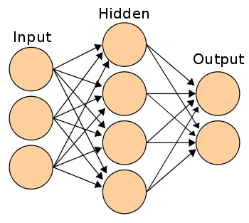
For those trying to deepen their understanding of neural nets, IAmTrask’s “A Neural Network in 11 lines of Python” is a staple piece. While it does a good job–a great job even–of helping people understand neural nets better, it still takes significant effort on the reader’s part to truly follow along.

My goal is to do more of the work for you and make it even easier. (Note: You still have to exert mental effort if you actually want to learn this stuff, no one can replace that process for you.) However I will try to make it as easy as possible. How will I do that? Primarily by taking his code and printing things, printing all the things. And renaming some of the variables to clearer names. I’ll do that too.

Link to my code: what I call the Annotated 11 line Neural Network.

First, let’s take a look at the inputs for out neural network, and the output we are trying to train it to predict:

Those are our inputs. As Mr. Trask points out in his article, notice the first column of the input data corresponds perfectly to the output. This does make this “classification task” trivial since there’s a perfect correlation between one of the inputs and the output, but that doesn’t mean we can’t learn from this example. It just means we should expect the weight corresponding to the first input column to be very large at the end of training. We’ll have to wait and see what the weights on the other inputs end up being.

In Mr. trask’s 1-layer NN, the weights are held in the variable syn0 (synapse 0). Read about the brain to learn why he calls them synapses. I’m going to refer to them as the weights, however.  Notice that we initialize the weights with random numbers that are supposed to have mean 0.

Let’s take a look at the initial values of the weights:

We see that they, in fact, do not have a mean of zero. Oh well, c’est la vie, the average won’t come out to be exactly zero every time.

Generating Our First Predictions

Let’s view the output of the NN variable-by-variable, iteration-by-iteration. We start with iteration #0.

Those are our inputs, same as from the chart above. They represent four training examples.

The first calculation we perform is the dot product of the inputs and the weights. I’m a crazy person (did I mention that?) so I’m going to follow along and perform this calculation by hand.

We’ve got a 4×3 matrix  (the inputs) and a 3×1 matrix (the weights), so the result of the matrix multiplication will be a 4×1 matrix.

We have:

I’m sorry I can’t create fancy graphics to show why those are the calculations you perform for this dot product. If you’re actually following along with this article, I trust you’ll figure it out. Read about matrix multiplication if you need more background.

Okay! We’ve got a 4×1 matrix of dot product results and if you’re like me, you probably have no idea why we got to where we’ve gotten, and where we’re going with this. Have patience for a couple more steps and I promise I’ll guide us to a reasonable “mini-result” and explain what just happened.

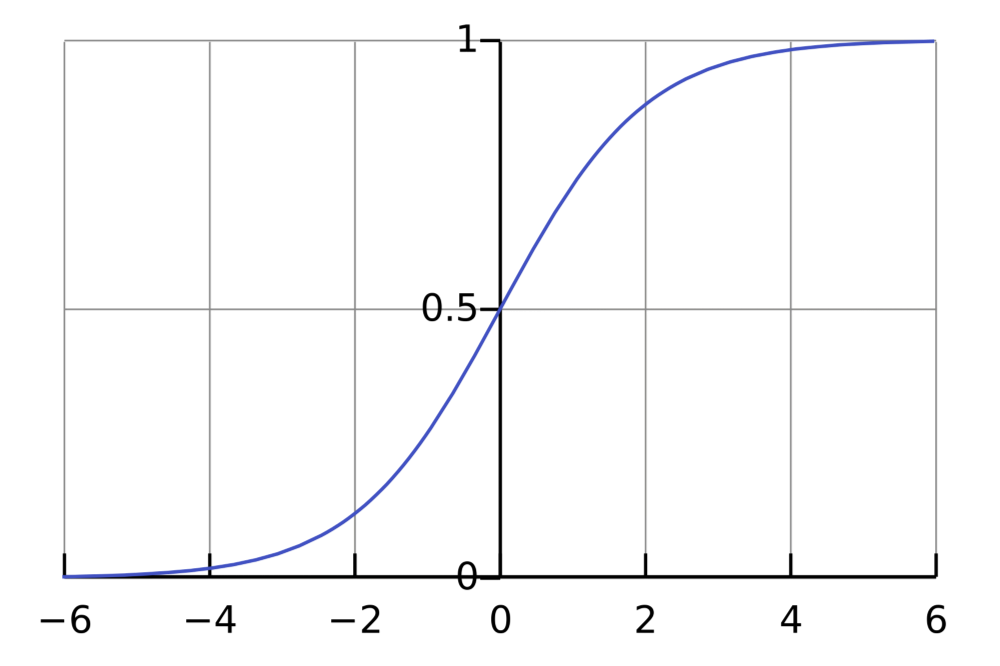
The next step according to the code is to send the four values through the sigmoid function. The purpose of this is to convert the raw numbers into probabilities (values between 0 and 1). This is the same step logistic regression takes to provide its classification probabilities.

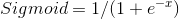
Element-wise, as it’s called in the world of matrix operations, we apply to the sigmoid function to each of the four results we got from the matrix multiplication*. Large values should be transformed close to 1. Large negative values should be transformed to something close to 0. And numbers in between should take on a value in between 0 and 1!

*I’m using the terms matrix multiplication and dot product interchangeably here.

Although I calculated the results of applying the sigmoid function “manually” in Excel, I’ll defer to the code results for this one:

So we take the results of the dot product (of the initial inputs and weights) and send them through the sigmoid function. The result is the “mini-result” I promised earlier and represents the model’s first predictions.

To be overly explicit, if you take the first dot product result, -.5463 and input it as the ‘x’ in the sigmoid function, the output is 0.3667.

This means that the neural network’s first “guesses” are that the first input has a 36.67% chance of being a 1. The second input has a 27% chance, the third a 46.17% chance, and the final and fourth input a 35.86% chance.

All of our dot product results were negative, so it makes sense that all of our predictions were under 50% (a dot product result of 0 would correspond to a 50% prediction, meaning the model has absolutely no idea whether to guess 0 or 1).

To provide some context, the sigmoid is far from the only function we could use to transform the dot product into probabilities, though it is the one with the nicest mathematical properties, namely that it is differentiable and its derivative, as we’ll see later, is mind-numbingly simple.