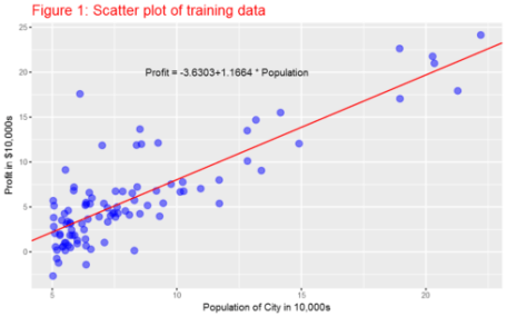
Plot the linear fitNow, since we know the parameters (slope and intercept), we can plot the linear fit on the scatter plot.
Here it is the plot:
[color=rgb(255, 255, 255) !important]
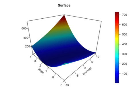
 Visualizing J(θ)
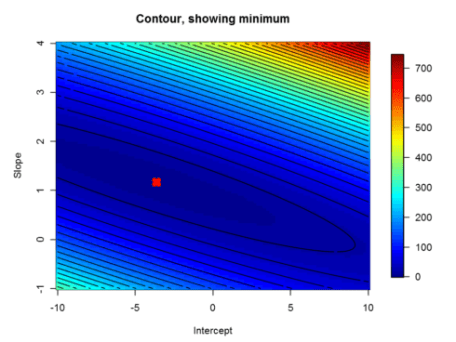
To understand the cost function J(θ) better, let’s now plot the cost over a 2-dimensional grid of θ0 and θ1 values. The global minimum is the optimal point for θ0 and θ1, and each step of gradient descent moves closer to this point.
Here it is the plot:
[color=rgb(255, 255, 255) !important]
 [color=rgb(255, 255, 255) !important]
 Normal Equation
Since linear regression has closed-form solution, we can solve it analytically and it is called normal equation. It is given by the formula below. we do not need to iterate or choose learning curve. However, we need to calculate inverse of a matrix , which make it slow if the number of records is very large. Gradient descent is applicable to other machine learning techniques as well. Further, gradient descent method is more appropriate even to linear regression when the number of observations is very large.
θ=(XTX)−1XTy
There is very small difference between the parameters we got from normal equation and using gradient descent. Let’s increase the number of iteration and see if they get closer to each other. I increased the number of iterations from 1500 to 15000.
As you can see, now the results from normal equation and gradient descent are the same.
Using caret packageBy the way, we can use packages develoed by experts in the field and perform our machine learning tasks. There are many machine learning packages in R for differnt types of machine learning tasks. To verify that we get the same results, let’s use the caret package, which is among the most commonly used machine learning packages in R.
Linear regression with multiple variablesIn this part of the exercise, we will implement linear regression with multiple variables to predict the prices of houses. Suppose you are selling your house and you want to know what a good market price would be. One way to do this is to first collect information on recent houses sold and make a model of housing prices. The file ex1data2.txt contains a training set of housing prices in Port- land, Oregon. The first column is the size of the house (in square feet), the second column is the number of bedrooms, and the third column is the price of the house.
Feature NormalizationHouse sizes are about 1000 times the number of bedrooms. When features differ by orders of magnitude, first performing feature scaling can make gradient descent converge much more quickly.
Gradient DescentPreviously, we implemented gradient descent on a univariate regression problem. The only difference now is that there is one more feature in the matrix X. The hypothesis function and the batch gradient descent update rule remain unchanged.
Normal Equation
Using caret package
SummaryIn this post, we saw how to implement numerical and analytical solutions to linear regression problems using R. We also used caret -the famous R machine learning package- to verify our results. The data sets are from the Coursera machine learning course offered by Andrew Ng. The course is offered with Matlab/Octave. I am doing the exercises in that course with R. You can get the code from this Github repository.


 扫码加好友,拉您进群
 全部版块
全部版块 我的主页
我的主页

 收藏
收藏