

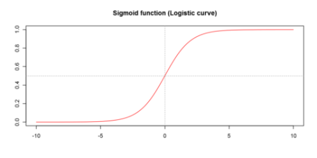
Logistic regression predicts the probability of the outcome being true. In this exercise, we will implement a logistic regression and apply it to two different data sets. The file ex2data1.txt contains the dataset for the first part of the exercise and ex2data2.txt is data that we will use in the second part of the exercise. To learn the basics of Logistic Regression in R read this post. In the first part of this exercise, we will build a logistic regression model to predict whether a student gets admitted into a university. Suppose that you are the administrator of a university department and you want to determine each applicant’s chance of admission based on their results on two exams. You have historical data from previous applicants that you can use as a training set for logistic regression. For each training example, you have the applicant’s scores on two exams and the admissions decision. Our task is to build a classification model that estimates an applicant’s probability of admission based the scores from those two exams. The first two columns contains the exam scores and the third column contains the label. Before starting to implement any learning algorithm, it is always good to visualize the data if possible. This is the plot: This is the formula: For large positive values of x, the sigmoid should be close to 1, while for large negative values, the sigmoid should be close to 0. Evaluating sigmoid(0) should give exactly 0.5. We can visualize the sigmoid function graphically: This is the plot: This is the formula: Initialize fitting parameters: The function below calculates cost. What is the cost for the initial theta parameters, which are all zeros? The function below calculates gradient. The gradient for the initial theta parameters, which are all zeros, is shown below We can use gradient descent to get the optimal theta values but using optimazation libraries converges quicker. So, let’s use the optim general-purpose Optimization in R to get the required theta values and the associated cost. Now, let’s plot the decision boundary. Only 2 points are required to define a line, so let’s choose two endpoints. This is the plot: After learning the parameters, you can use the model to predict whether a particular student will be admitted. For example, for a student with an Exam 1 score of 45 and an Exam 2 score of 85, the probability of admission is shown below. Now, let’s calculate the model accuracy. Let’s use a threshould of 0.5. In this part of the exercise, we will implement regularized logistic regression to predict whether microchips from a fabrication plant passes quality assurance (QA). During QA, each microchip goes through various tests to ensure it is functioning correctly. Suppose you are the product manager of the factory and you have the test results for some microchips on two different tests. From these two tests, you would like to determine whether the microchips should be accepted or rejected. This is the plot: The above figure shows that our dataset cannot be separated into positive and negative examples by a straight-line through the plot. Therefore, a straightforward application of logistic regression will not perform well on this dataset since logistic regression will only be able to find a linear decision boundary.本帖隐藏的内容
Load the data and display first 6 observations
Visualizing the data


Let’s code the sigmoid function so that we can call it in the rest of our programs.
Let’s check!
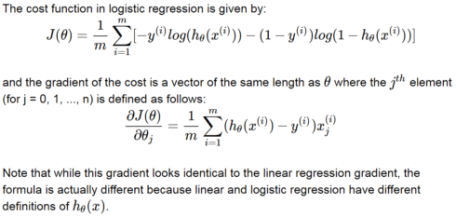
Cost function and gradient
Add ones for the intercept term:
General-purpose Optimization in lieu of Gradient Descent
Decision Boundary

Evaluating logistic regression
Model accuracy
Regularized logistic regression

One way to fit the data better is to create more features from each data point. Let’s map the features into all polynomial terms of x1 and x2 up to the sixth power.
new_data=c() for(i in 1:6){ for(j in 0:i){ temp= (ex2data2$Test1)^i+(ex2data2$Test2)^(i-j) new_data=cbind(new_data,temp) } } colnames(new_data)=paste0("V",1:ncol(new_data))head(new_data) V1 V2 V3 V4 V5 V6 V7 V8 V9 V10 ... V18 V19 V20 V21 V22 V23 V24 V25 V26 V27 0.750827 1.051267 0.4920125 0.7021883 1.002628 0.34248835 0.48951894 0.69969475 1.0001347 0.23950380 ... 0.489384548 0.6995604 1.0000004 0.11720601 0.16754246 0.23949691 0.34235362 0.48938421 0.6995600 1.000000 0.592198 0.907258 0.4777439 0.6935411 1.008601 0.32053699 0.46834512 0.68414232 0.9992023 0.22016895 ... 0.469135943 0.6849331 0.9999931 0.10325661 0.15075249 0.22009561 0.32133531 0.46914344 0.6849406 1.000001 0.478540 0.786290 0.5248820 0.7379220 1.045672 0.32197261 0.46944951 0.68248944 0.9902394 0.23172821 ... 0.478764279 0.6918042 0.9995542 0.11014216 0.15906514 0.22973755 0.33182843 0.47930533 0.6923453 1.000095 0.127190 0.625000 0.3928198 0.6428150 1.140625 0.07391533 0.19946042 0.44945563 0.9472656 0.08337761 ... 0.244779025 0.4947742 0.9925842 0.01882106 0.03472131 0.06638313 0.12943062 0.25497571 0.5049709 1.002781 -0.047610 0.486750 0.4802462 0.7290656 1.263426 -0.03424282 0.08161744 0.33043683 0.8647968 0.11640420 ... 0.181204639 0.4300240 0.9643840 0.02847289 0.04017018 0.06529107 0.11924025 0.23510051 0.4839199 1.018280 -0.314970 0.475230 0.3193996 0.4851836 1.275384 -0.13527846 -0.10049699 0.06528697 0.8554870 0.07777351 ... 0.004219529 0.1700035 0.9602035 0.02096929 0.02129048 0.02282143 0.03011858 0.06490005 0.2306840 1.020884 y=ex2data2$Label X=new_dataAs a result of this mapping, our vector of two features (the scores on two QA tests) has been transformed into a 28-dimensional vector. A logistic regression classifier trained on this higher-dimension feature vector will have a more complex decision boundary and will appear nonlinear when drawn in our 2-dimensional plot. While the feature mapping allows us to build a more expressive classifier, it also more susceptible to overfitting. In the next parts of the exercise, we will implement regularized logistic regression to fit the data and also see for ourselves how regularization can help combat the overfitting problem.
my_cost2=function(theta, X, y,lambda){ cost_gradient=list() # cost_and_gradient compute cost and gradient for logistic regression using theta h_theta= my_sigmoid(X%*%theta) cost= 1/nrow(X)*sum(-y*log(h_theta)-(1-y)*log(1-h_theta))+lambda/(2*nrow(X))*sum(theta^2) return(cost) } my_gradient2=function(theta, X, y,lambda){ h_theta= my_sigmoid(X%*%theta) ## OPTION 1-- looping gradient=rep(0,ncol(X)) for(j in 2:ncol(X)){ for(i in 1:nrow(X)){ gradient[1]=gradient[1]+1/nrow(X)*(my_sigmoid(X[i,]%*%theta)-y)*X[i,1] gradient[j]=gradient[j]+1/nrow(X)*(my_sigmoid(X[i,]%*%theta)-y)*X[i,j]+lambda/(nrow(X))*theta[j] } } # option2-more succint # gradient= 1/nrow(X)*(my_sigmoid(t(theta)%*%t(X))-t(y))%*%X+(lambda/(nrow(X)))*c(0,theta[-1]) return(gradient) }Let’s initialize theta:
initial_theta =matrix(rep(0,ncol(X)))What is the cost for the initial theta?
round(my_cost2(initial_theta,X,y,lambda=10),3) 0.693OptimizationNow, since we have the cost function that we want to optimize and the gradient, we can use the optimization function optim to find the optimal theta values.
We have to try various values of lambda and select the best lambda based on cross-validation. But for now, let’s just take lambda=1.
The theta values from the optimization are shown below.
matrix(as.vector(optimized$par),ncol=9) 0.49507083 -0.05202124 -0.08527443 -0.1575100 -0.035020544 -0.11079198 0.01169745 -0.12174228 -0.12234383 0.05639364 -0.02062364 0.01959276 -0.1129876 -0.003622936 -0.06626957 0.04309506 -0.13996607 -0.01747664 -0.15688844 -0.05837426 0.05099037 -0.1398877 -0.092568188 -0.09316975 -0.14349836 -0.09544366 0.01392097 ex2data2$fitted_result=my_sigmoid(X%*%optimized$par)Let’s use a threshold of 0.5.
ex2data2$fitted_result_label=ifelse(ex2data2$fitted_result>=0.5,1,0) head(ex2data2,10) Test1 Test2 Label fitted_result fitted_result_label 0.051267 0.699560 1 0.4765027 0 -0.092742 0.684940 1 0.4629791 0 -0.213710 0.692250 1 0.4410811 0 -0.375000 0.502190 1 0.4701446 0 -0.513250 0.465640 1 0.4459059 0 -0.524770 0.209800 1 0.4554844 0 -0.398040 0.034357 1 0.4730207 0 -0.305880 -0.192250 1 0.4618593 0 0.016705 -0.404240 1 0.4735035 0 0.131910 -0.513890 1 0.4640032 0 Evaluating the fitNow, we can evaluate the fit by calculating various metrics such as F1 score, precision and recall. Let’s just see accuracy here. You can see the values of the other metrics here.
accuracy=sum(ex2data2$Label==ex2data2$fitted_result_label)/nrow(ex2data2) cat("The accuracy is: ") round(accuracy,3) The accuracy is: 0.653 SummaryLogistic regression is a classification machine learning technique. In this blog post, we saw how to implement logistic regression with and without regularization. In the first part, we used it to predict if a student will be admitted to a university and in the second part, we used it to predict whether microchips from a fabrication plant pass quality assurance. We used special optimization function in lieu of gradient descent to get the optimal values of the coefficients. The data sets are from the Coursera machine learning course offered by Andrew Ng. The course is offered with Matlab/Octave. I am doing the exercises in that course with R. You can get the code from this Github repository.
 扫码加好友,拉您进群


 收藏
收藏

